Random number generators, deterministic systems and the difficulty of modeling stochasticity

13 Apr 2022

When using the R language I decided to look up the documentation of the Random function which actually seems to be quite interesting. This Random function in the R base library offers several different pseudorandom number generators: the Wichmann-Hill, Marsaglia-Multicarry, Super Duper, Mersenne-Twister, Knuth-TAOCP-2002, Knuth-TAOCP, and L’Ecuyer-CMRG.

Another blog I found has summarized the apparent performance advantages and disadvantages of each of these random number generators (RNGs) so I will link it here. The data in the post is taken from L’Ecuyer and Simard, 2007.

Firstly some overall philosophical notes about the nature of computers as deterministic state machines. It is interesting that such machines require algorithms such as these to even attempt to simulate stochastic behavior! One thinks of human beings as the opposite of computers: it is easier for us to be “stochastic” and it is hard for us to be reliably “deterministic” and implement (for most people) complex algorithms mentally in an efficient manner. In contrast, a computer in the macro sense can only have a certain amount of states, such that we can consider each possible arrangement of bytes at a given moment in CPU registers, in main memory, in storage etc, to be a finite (though large) number of possible states. That is, (classical) computers suffer a discreteness limitation, as their fundamental operation requires this in accordance with their theoretical model of binary logic, as well as the practical implementation of this.

One notes that (pseudo) RNGs tend to utilize certain “seeds” or certain input values to be fed into RNG algorithms to produce a given pseudorandom number. This tends to be something such as the timestamp (which can reliably be said to different between every usage) although this does not prevent certain problems. Some criticisms have been noted for example of the default rand() function in many C implementations such as that in glibc. The implementation in musl is quite simple:

#include <stdlib.h>
#include <stdint.h>

static uint64_t seed;

void srand(unsigned s)
{
    seed = s-1;
}

int rand(void)
{
    seed = 6364136223846793005ULL*seed + 1;
    return seed>>33;
}

The method utlized by musl appears to be a linear congruential generator, whereas the reference implementation is by Knuth. It is noted that LCGs are not sufficiently secure for “cryptographic applications”. The algorithm follows the formula:

$$X_{i+1} = (aX_i + c) \mod m, i=0,1,2,...$$

Here a is the constant multiplier, c is the increment, m is the modulus, hence in the above musl implementation, the multiplier is 6364136223846793005, the increment is 1, and the modulus is 2⁶⁴.

The glibc random() code is interesting because it provides very extensive comments. The code comments note:

In addition to the standard rand()/srand() like interface, this package also has a special state info interface. The initstate() routine is called with a seed, an array of bytes, and a count of how many bytes are being passed in; this array is then initialized to contain information for random number generation with that much state information. Good sizes for the amount of state information are 32, 64, 128, and 256 bytes. The state can be switched by calling the setstate() function with the same array as was initialized with initstate(). By default, the package runs with 128 bytes of state information and generates far better random numbers than a linear congruential generator. If the amount of state information is less than 32 bytes, a simple linear congruential R.N.G. is used.

What method is utilized instead of a linear congruential RNG?

The random number generation technique is a linear feedback shift register approach, employing trinomials (since there are fewer terms to sum up that way).

The man page states:

The random() function uses a nonlinear additive feedback random number generator employing a default table of size 31 long integers to return successive pseudo-random numbers in the range from 0 to RAND_MAX. The period of this random number generator is very large, approximately 16 * ((2^31) - 1).

In the code we observe the table:

static int32_t randtbl[DEG_3 + 1] =
  {
    TYPE_3,
    -1726662223, 379960547, 1735697613, 1040273694, 1313901226,
    1627687941, -179304937, -2073333483, 1780058412, -1989503057,
    -615974602, 344556628, 939512070, -1249116260, 1507946756,
    -812545463, 154635395, 1388815473, -1926676823, 525320961,
    -1009028674, 968117788, -123449607, 1284210865, 435012392,
    -2017506339, -911064859, -370259173, 1132637927, 1398500161,
    -205601318,
  };

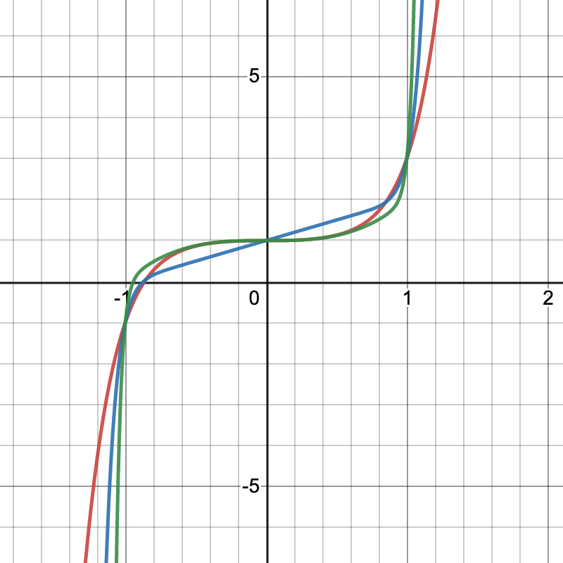
Which such trinomials are utilized? The code details 4 types of RNGs, with TYPE_0 being the simple linear congruential method, the others being trinomials: TYPE_1 $x^7 + x^3 + 1$, TYPE_2 $x^15 + x + 1$, and TYPE_3 $x^31 + x^3 + 1$. These three trinomial equations intersect at the points (0,1), (1,3) and (-1,-1), while additional intersections exist between the pairs at non-integer points:

These trinomials are important enough that lists have been published of them and they have been subject of study.

The method utilized by glibc in random_r() involves the formula:

int32_t val = ((state[0] * 1103515245U) + 12345U) & 0x7fffffff;

In the GNU man page is detailed the differences between random() and random_r():

The random_r() function is like random(3), except that instead of using state information maintained in a global variable, it uses the state information in the argument pointed to by buf, which must have been previously initialized by initstate_r(). The generated random number is returned in the argument result.

A linear feedback shift register utilizes “a linear function of its previous state” as the input bit.

Another set of random number generators in UNIX and UNIX-like systems (such as macOS, BSD, Linux) occurs in the exposed /dev/random and /dev/urandom “files”. Under the UNIX paradigm “everything is a file” so these “files” can be handled by utilities such as cat as if they were files, allowing pipelining to files etc. These produce continuous streams of random bytes which are considered “cryptographically secure”.

Let’s examine the randomness tests contained within the TestU01 suite proposed by L’Ecuyer and Simard, 2007. They first define a “good imitation” of “independent uniform random variables” (colloquially, what we would presumably consider “truly random”):

RNGs for all types of applications are designed so that their output sequence is a good imitation of a sequence of independent uniform random variables, usually over the real interval $(0, 1)$ or over the binary set $\{0, 1\}$. In the first case, the relevant hypothesis $H_0^A$ to be tested is that the successive output values of the RNG, say $u_0 , u_1 , u_2 , . . .$, are independent random variables from the uniform distribution over the interval $(0, 1)$, that is, i.i.d. $U (0, 1)$. In the second case, $H_0^B$ says that we have a sequence of independent random bits, each taking the value 0 or 1 with equal probabilities independently of the others.

The paper discusses many methods of testing (implemented in their testing suite), a few are given below:

1. Statistical two-level statistical test

   Several authors have advocated and/or applied a two-level (or second-order) procedure for testing RNGs [Fishman 1996; Knuth 1998; L’Ecuyer 1992; Marsaglia 1985]. The idea is to generate N “independent” copies of Y , say $Y_1 , . . . , Y_N$, by replicating the first-order test N times on disjoint subsequences of the generator’s output. Let F be the theoretical distribution function of Y under $H_0$. If F is continuous, the transformed observations $U_1 = F (Y_1)$, . . . , $U_N = F (Y_N )$ are i.i.d. $U (0, 1)$ random variables under $H_0$ . One way of performing the two-level test is to compare the empirical distribution of these $U_j$ ’s to the uniform distribution, via a goodness-of-fit (GOF) test such as those of Kolmogorov- Smirnov, Anderson-Darling, Crámer-von Mises, etc.
   […]
   The p-value of the GOF test statistic is computed and $H_0$ is rejected if this p-value is deemed too extreme, as usual.

2. Testing a stream of real numbers, this involves “measuring global uniformity”, “measuring clustering” (if the numbers tend to be clustered in a certain manner), and “run and gap tests” (counts gap between successive values that land in a certain interval, using the heuristic of Lebesgue measure).

3. “Testing for n subsequences of length t”

Blackman and Vigna, 2018 discuss some of the weaknesses of “F₂-linear pseudorandom number generators”. They propose a new generator called xoshiro256** which supposedly addresses the failures of previous RNGs including their own Xoshiro128+. This in turn was criticized by O’Neill, 2018, where she compares it to her own PCG random number generator algorithms.